

Charts and analytics
An analytic is a chart (or a row of figures, or a table) worked out from your live schedule: labor hours per week against what your crew can work, an S-curve of planned against earned progress, activities by total float, the forecast finish across every update. Analytics re-run whenever the schedule changes, so nothing is ever exported and pasted.
You can build one yourself in the analytic editor, but the quickest way is to describe it to Owl. Owl writes the analytic, checks the numbers, and opens it in its own tab.
What an analytic is made of
Every analytic is the same four parts, read in the same order as the chart:
| Part | What it says | Example |
|---|---|---|
| X axis | What runs along the bottom. | Dates by week, WBS phases, schedule updates |
| Series | Each thing drawn on it: a value, how it's shown, how it's drawn, and (for one series) what splits it. | Planned hours per week, drawn as steps, by resource |
| Compare with | Another schedule to draw every series on too. | The baseline, a named revision, a scenario |
| Filter | Which activities count. | Only critical work, only open activities |
The x axis can be:
- Dates — the schedule's timeline, by day, week, month, quarter or year. A lookahead limits it to a number of days from the data date.
- A field — one bar per value of a field: a WBS level, a task code, status, resource.
- Ranges of a number — a histogram, such as activities by total float.
- Schedule updates — one point per update, for trends like the forecast finish.
- Each activity — one row per activity, a table (a lookahead list, milestones against the baseline).
- Nothing — no axis, just figures: a row of KPI tiles.
Note: Owl works out the axes for you. The first unit drawn (hours, days, dollars) reads on the left axis, a second unit gets a right axis. A third unit is refused with a suggestion, such as showing it as a % of its total.
Ask Owl for an analytic
Say what to measure, how to group it, and what to compare it with. Owl builds the analytic, runs it, reads the numbers back to you, and points out anything odd it sees in them.
The analytic below came from one message: "Chart planned labor hours per week by resource against available hours, compared with the Derisked Schedule scenario. Put it on a new dashboard called Crew Planning." Owl added it to the Analytics list, made the Crew Planning dashboard, and explained what it found: the peak week runs well over the crew's available hours, and in the Derisked Schedule the same peak moves about nine weeks later.
New analytics and dashboards appear in the project tree as soon as Owl makes them, and an analytic that is already open updates in place when Owl changes it.
Read an analytic
Open any analytic from Analytics in the project tree. It opens in its own tab: the chart in the middle, the numbers under it, and the editor on the right.
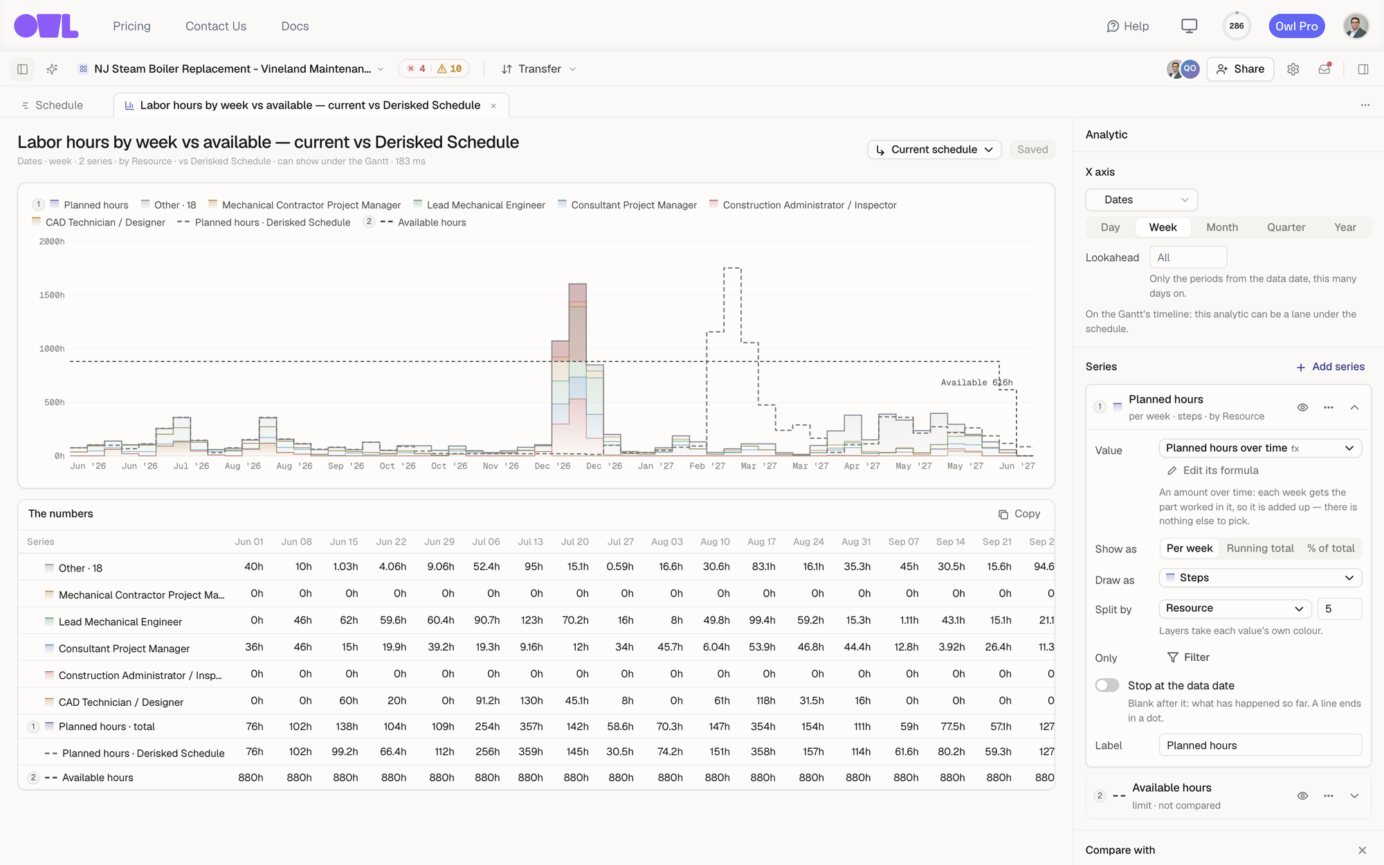 12345671The title and a one-line summary of the spec: Dates · week · 2 series · by Resource · vs Derisked Schedule · can show under the Gantt.2Current schedule runs the whole analytic on a scenario instead.3The chart. Each series is numbered in the legend: 1 planned hours, split by resource, with its Derisked Schedule ghost (dashed), and 2 available hours, drawn as a limit.4The numbers — every value the chart draws, period by period. Copy puts them on your clipboard for a spreadsheet.5X axis — dates by week, with an optional lookahead.6A series card: its value, how it's shown, how it's drawn, and what splits it.7Compare with — another schedule, further down the editor.
A few things to look for:
- The legend numbers (1, 2, 3) match the series cards in the editor and the rows of The numbers.
- A dashed line or outline is the compared schedule — here, the Derisked Schedule's total hours each week.
- A limit is a ceiling drawn as a dashed step, labeled at its end ("Available 616h"); whatever stacks above it is over capacity.
- The summary line under the title says, in words, what the analytic is: its axis, how many series, what it's split by and compared with, and whether it can be a lane under the Gantt.
Change an analytic in the editor
Every change shows up in the chart straight away. Nothing is stored until you click Save changes (or Save analytic for a new one). To start from scratch, use the + on Analytics in the project tree, or Add analytic → New analytic… on a dashboard.
Series
Click Add series to add one. You can start from:
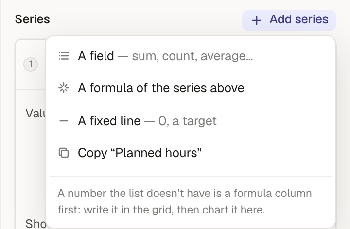 The Add series menu: A field, A formula of the series above, A fixed line, and Copy the selected series.
- A field — a sum, count or average of something in the schedule: activity counts, durations, float, planned hours, cost.
- A formula of the series above — a value worked out from the other series, point by point. With series named
evandpv, the formula[ev] / [pv]gives each month's ratio. - A fixed line — a target or a zero line.
- Copy — a copy of an existing series, to change one thing about it.
Each series card then has:
- Value — what is added up. Values over time, such as Planned hours over time, come from formula columns; Edit its formula opens the formula above the chart.
- Show as — Per week (each period's own amount), Running total, or % of total (the running total as a share of its own total, or of another series' total: that's how an S-curve shows earned as a percent of planned).
- Draw as — how it's drawn. Options that don't fit the series are greyed out with the reason.
- Split by — layers the series by a field (resource, status, a WBS level, a task code) and keeps the top few values, with the rest in Other. Only one series per analytic can be split.
- Only — a filter for this series alone, on top of the analytic's filter.
- Stop at the data date — leaves the series blank after the data date, for what has actually happened.
- Label — the name in the legend.
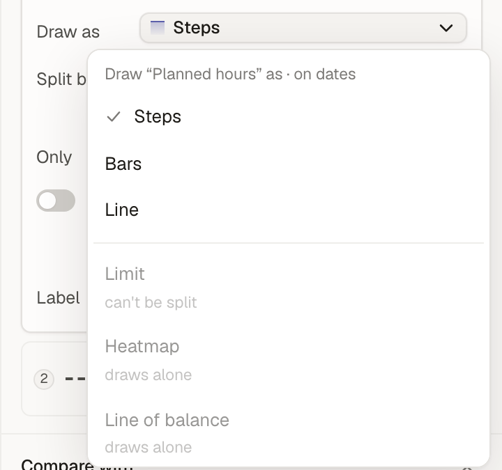 The Draw as menu for a series on dates: Steps, Bars and Line, with Limit, Heatmap and Line of balance greyed out and the reason under each.
The ways to draw a series:
| Draw as | Use it for |
|---|---|
| Steps | Amounts that belong to a whole period, like hours per week. Split layers stack. |
| Bars | Separate bars per period or per value. |
| Line | S-curves, trends and ratios. |
| Limit | A ceiling such as available hours. Anything stacked above it is shaded as over. |
| Heatmap | One row per value of the split against time; darker means more. |
| Line of balance | Each location's first start to last finish over time (split by an ordered location field). |
| Share | Parts of one whole as a single 100% bar. |
| Tile | A single figure, with its change since the last update and against the compared schedule. |
| Column | A column in a table of activities. |
| Range | Each milestone's finish against the compared schedule, or a simulation's P10–P90 when it compares with one. |
Values over time
A value that changes over time — hours per week, cost per month, earned progress — is a formula column made with SPREAD. Every project starts with these, and you can open and change them like any formula column:
| Column | What it spreads over time |
|---|---|
| Duration over time | Each activity's duration over its working days (the planned S-curve). |
| Late duration over time | The same over its late dates. |
| Earned duration over time | The done part of each activity, up to the data date. |
| Planned hours / cost over time | Each assignment's hours (and hours × rate) over the activity's working days. |
| Actual hours / cost over time | Hours and cost spent so far, over the actual dates. |
| Forecast hours over time | Hours spent where they were spent, plus what's left from the data date on. |
| Available hours over time | Each labor resource's working hours over the project, times its max units per time (a crew of three has three times the hours): the limit planned hours are drawn under. |
Planned hours over time, for example, is:
SPREAD([Budgeted units], Task[Start date], Task[Finish date])
each assignment's hours spread evenly over its activity's working days. Anything you can write as a column over time, you can chart. See Values over time for how SPREAD and its relatives work.
Tip: If the number you want isn't in the field list, make a formula column for it first in the grid (Columns, filters, colors and views), then chart that column.
Compare with another schedule
Under Compare with, click Add and pick a schedule. Every series is worked out again on that schedule, by the same engine, from its own activities and assignments, and drawn beside itself.
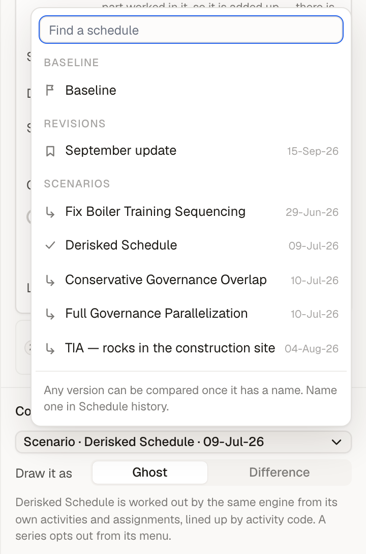 121Pick the Baseline, a named revision, or a scenario.2Ghost draws the other schedule beside each series (a dashed line or outline); Difference draws this schedule minus that one.
- Baseline — the plan of record.
- Revisions — any version of the schedule once it has a name in Schedule history.
- Scenarios — a what-if copy of the schedule (see Explore what-if scenarios).
A limit, and any series you take out from its ⋯ menu, is never compared. Over Schedule updates there is nothing to compare with: the history already is the comparison.
Filter
Filter at the bottom of the editor limits every series to the activities you choose, with the same filter builder as the schedule. On a dashboard, the dashboard's own filter is added to it.
Show an analytic under the Gantt
An analytic over dates, drawn as steps, bars, lines or limits, can be a lane under the Gantt, lined up with the timeline above it. The analytic's summary line says can show under the Gantt when it qualifies.
Open Lanes on the schedule toolbar and tick the analytics you want. Lanes that are on come first; drag them to reorder. The ones that can't be lanes are listed greyed out, each with the reason ("x is a field", "draws a heatmap").
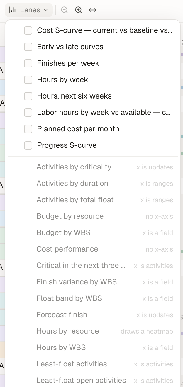 The Lanes menu: eight analytics over dates that can be lanes, and the rest greyed out with the reason each can't.
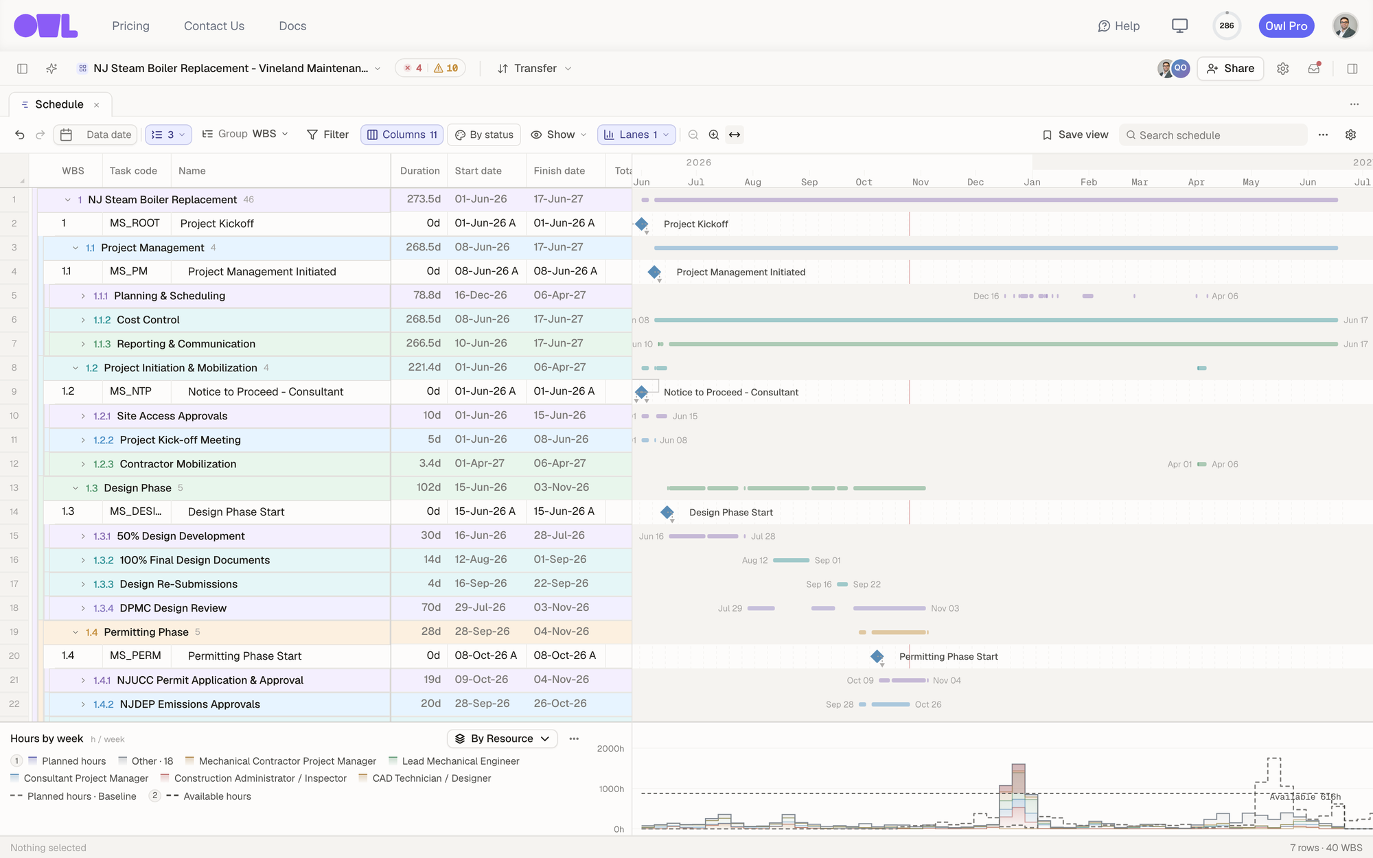 1231Lanes on the toolbar turns lanes on and off (here 1 is on).2The lane uses the Gantt's own timeline, so the December peak sits under the work that causes it.3Change the split right on the lane.
Lanes are saved with your saved view, so a "Resource loading" view can open with its lanes already on.
Put analytics on a dashboard
A dashboard arranges several analytics on one page with shared controls: run them all against a scenario, or filter them all at once. Dashboards are covered in Create custom dashboards.
What to do next
- Build a standing view — Create custom dashboards.
- Track cost — Track cost and schedule with EVM.
- Measure a what-if — Analyze a scenario.
- Write the columns behind a chart — Values over time.